HPP Blog #1: Python Profiling
In this post, which will be the first in a series, I will go over the basics of Python profiling in a way that you were probably never taught in school! I was never taught this explicitly, and only through interactions with people much smarter than me did I recognize its importance.
Why is Profiling Important?
At the moment, these are the reasons why I personally think profiling is becoming more important:
- Don't over-optimize the wrong thing. Most problems have several approaches with very different ceilings. Meticulous tuning of a weak solution rarely beats starting with a better design. Profile to see which path deserves the effort.
- Fix what you believe is the problem. Oftentimes, you skip profiling and guess, but for a program of any significant complexity, you will probably fix the wrong thing. Profiling oftentimes can actually be the "lazy" and more efficient solution. Don't spend hours speeding up a part of your code that's already fast, only to realize that the slowest part was somewhere else instead.
- Rise of vibe coding. Vibe coding/AI coding is not inherently bad, but, due to the inherent stochastic nature of LLMs, you're probably getting a very suboptimal initial solution, that you may not even understand is bad.
As a heads-up, the implementation that is used here is deliberately the simplest/least-optimal one. Feel free to follow along in this jupyter notebook.
Print & Time Statements
The simplest way to profile would most definitely be to just use time and print statements. Print statements are already super useful in debugging, so why not profiling as well?
The simplest way to go about using time and print statements is simply something along the lines of:
t1 = time.time()
result = fn(*args, **kwargs)
t2 = time.time()
print(f"Function took {t2-t1} seconds")
A better way of doing this is to define some type of decorator in order to automate our timing measurements.
from functools import wraps

def timePrintFn(fn):
    @wraps(fn)
    def wrapper(*args, **kwargs):
        start = time.time()
        result = fn(*args, **kwargs)
        end = time.time()
        print(f"{fn.__name__} took {end-start:.4f} seconds")
        return result
    return wrapper
Of note, on other texts, such as the textbook High Performance Python, there is a reference to the decorator being slightly faster, however, this is likely just noise in the measurement and doesn't seem to consistently be the case. In fact, it is the other way around, the decorator adds additional function overhead and thus should be slightly slower. Individual test cases may appear faster/slower when comparing the two because of statistical noise, but averaged over long time-series the decorator should be, on-average, slower.
Another general method for doing this is using the %timeit
method. The %timeit
method is simply using the Python command and running it in the command line.
With two major flags, you choose how many times to call the function consecutively
where the final time is the total time for all the calls divided by the number
of calls. Then you specify the number of runs which is the number of times
the above operation is conducted.
N = 1  # of times run consecutively per run
R = 1  # of runs

%timeit -n N -r R multiply_matrices_pure_python(matrix_a, matrix_b)
This then returns the fastest of all the runs, or the outer loop.
You can also try %%time, which basically times an entire cell
in a jupyter notebook.
First, when measuring functions this way, it's helpful to remove the first test-case time because of import statements and other noise present in the first measurement. A warm-up run of the function/code is helpful to run before actual testing. Then you should run it a couple of times, usually around 5, depending on what the use case is of course, and how fast you want results.
cProfile
cProfile is the faster of the two profilers in the standard Python library because it's written in C.
Before you profile anything, you should probably first make a guess, or hypothesis, about the speed of different parts of your code. This helps you figure out where you are consistently wrong at guessing the speed of a program and improves your coding intuition.
One of the ways to use cProfile is as a command-line argument. The CLI definition can be found here but the general gist is:
$ python -m cProfile [options] script.py [script_args...]The one that I think is most useful is to use the cumulative flag, which gets you the total time spent within a specific function.
$ python -m cProfile -s cumulative script.py [script_args...]If you are in the repo, and run it on the matmul.py script, you will get something like this:
$ USER Profiling % python -m cProfile -s cumulative matmul.py
Generating two 1000x1000 matrices...
Sample from matrix A (top-left 3x3):
[56, 77, 49]
[74, 21, 89]
[19, 57, 31]
Sample from matrix B (top-left 3x3):
[25, 11, 37]
[13, 58, 50]
[55, 98, 21]
Starting matrix multiplication...
Matrix multiplication completed!
Result matrix size: 1000x1000
Sample from result matrix (top-left 3x3):
[2488413, 2460504, 2424927]
[2501376, 2440835, 2462731]
[2465470, 2417773, 2460009]
         16539727 function calls (16539695 primitive calls) in 123.430 seconds

   Ordered by: cumulative time

   ncalls  tottime  percall  cumtime  percall filename:lineno(function)
      3/1    0.000    0.000  123.457  123.457 {built-in method builtins.exec}
        1    0.007    0.007  123.457  123.457 matmul.py:1()
        1    0.000    0.000  123.444  123.444 matmul.py:55(main)
        1  121.197  121.197  121.224  121.224 matmul.py:26(multiply_matrices_pure_python)
        2    0.001    0.001    2.220    1.110 matmul.py:9(generate_matrix)
     2000    0.258    0.000    2.219    0.001 matmul.py:21()
  2000000    0.302    0.000    1.961    0.000 random.py:358(randint)
  2000000    0.806    0.000    1.659    0.000 random.py:284(randrange)
  2000000    0.513    0.000    0.673    0.000 random.py:235(_randbelow_with_getrandbits)
  6000000    0.180    0.000    0.180    0.000 {built-in method _operator.index}
  2534239    0.094    0.000    0.094    0.000 {method 'getrandbits' of '_random.Random' objects}
  2000000    0.066    0.000    0.066    0.000 {method 'bit_length' of 'int' objects}
        1    0.001    0.001    0.027    0.027 matmul.py:41()
      6/1    0.000    0.000    0.005    0.005 :1167(_find_and_load)
      6/1    0.000    0.000    0.005    0.005 :1122(_find_and_load_unlocked)
If you compare, we've about doubled our time (this new one took ~120 seconds) just simply because we are profiling the script itself. As we've sorted by execution time, we can assess where it's mostly spent. Here is how to go about reading this:
- ncalls: total number of calls. The first number is the total number of calls, while the second number is the primitive calls––basically any call that was not recursive
- tottime: time spent in that function excluding the function call itself
- percall: tottime/ncalls
- cumtime: across all sub-functions called included
- percall: cumtime/ncalls
Looking at the above code, it's clear that the heavy lifting is being done primarily by the multiply_matrices which makes sense as it's 121 seconds. Also because tottime ≈ cumtime, we can see that it's not calling expensive functions, and most of the work is being done in these nested for-loops which is crushing the performance. We can also read the matrix generation runs, which call the generate_matrix and other which is relatively costly, but costly because of calls to other operations due to the delta in the tottime and cumtime values. It's clear that in the generation, randrange is the most expensive step as well, with each step adding a little bit of overhead.
Then to get further analysis, we can run the following to save it into a statistics folder:
$ python -m cProfile -o matmul.stats matmul.pyAfter doing this, feel free to check out the jupyter notebook on
profiling. Then afterwards you can see that we can call print_callers()
as well as print_callees(). This gives you a list on the left
of which functions called which other functions and how many times and
vice versa. The caller and callees list may be extremely helpful when
looking for cached calls or when something is called much more than you
would expect.
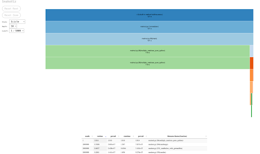
SnakeViz
SnakeViz is a way to draw the output of cProfile as flame graph. The larger the box, the longer that specific part of the code takes to run. This package you need to:
$ pip install snakevizThen run !snakeviz in jupyter notebook or then calling it in CLI
in the following form:
$ snakeviz matmul.prof
# Or
$ snakeviz matmul.stat
You can then sort by various strategies like cumtime, percall, or ncalls.
Line Profiler
Line profiler is more granular method of profiling functions, and works by going line-by-line. Use it primarily as a tool for profiling after determining which functions you need to understand more.
To use it. First install:
$ pip install line_profilerThen mark the function you want to profile with the decorator @profile, then run it with the following command (details
here):
$ kernprof -l -v matmul_line_profiler.pyOf note, this takes significantly more time, so you may want to edit the original script to use a 300 × 300 matrix instead for the multiplication. Here is what the output looks like for a simple example:
Total time: 13.9963 s
File: matmul_line_profiler.py
Function: multiply_matrices_pure_python at line 25

Line #      Hits         Time  Per Hit   % Time  Line Contents
==============================================================
    25                                           @profile
    26                                           def multiply_matrices_pure_python(A, B):
    27                                               """
    28                                               Multiplies two matrices using pure Python nested loops.
    29
    30                                               Args:
    31                                                   A (list): First matrix (2D list)
    32                                                   B (list): Second matrix (2D list)
    33
    34                                               Returns:
    35                                                   list: Result matrix C where C = A * B
    36                                               """
    37                                               # Get the size of the matrices (assuming they are square and of the same size)
    38         1          1.0      1.0      0.0      size = len(A)
    39
    40                                               # Initialize the result matrix with zeros
    41         1       1400.0   1400.0      0.0      C = [[0 for _ in range(size)] for _ in range(size)]
    42
    43                                               # Perform matrix multiplication
    44                                               # Iterate through rows of A
    45       301        329.0      1.1      0.0      for i in range(size):
    46                                                   # Iterate through columns of B
    47     90300      22110.0      0.2      0.2          for j in range(size):
    48                                                       # Iterate through rows of B
    49  27090000    6350531.0      0.2     45.4              for k in range(size):
    50  27000000    7621961.0      0.3     54.5                  C[i][j] += A[i][k] * B[k][j]
    51
    52         1          6.0      6.0      0.0      return C
How do we read this?
- Line #: The line number in the source file
- Hits: Basically how many times this particular line was run
- Time: Amount of time units is an arbitrary measurement (different OSes use diff measurements), this is useful for comparing different lines, and also you can calculate the exact units by comparing with the total time.
- Per Hit: Time / Hits, basically how many time units per hit took on average.
- % Time: what percentage of the total time was spent in this line.
Afterwards, if you want even more granular flow, for different programs,
it's possible that the program can be rewritten in as to break up
different steps or converting each line into it's own unit. Such as
breaking up any ands and or statements in a way that allows you to, more
easily, dissect the counts. Afterwards, you can also test individual lines
or components with the
%timeit components.
Memory Profiler
Memory usage helps you 1. Minimize RAM usage and 2. Optimize RAM vs. CPU cycles (i.e. determining if RAM caching makes sense). Memory profiler is similar but slower than line profiler. Memory profiling is generally much less clear-cut than line profiling. In general, it is much harder to pinpoint why/where memory is allocated for what, and it's difficult to see cascading effects. Instead, focus on hot spots and trends rather than line by line.
To use it. First install it using:
$ pip install memory_profilerYou use the same @profile header as before. So simply call:
$ python -m memory_profiler matmul_profiler.pyThe result looks something like this:
Line #    Mem usage    Increment  Occurrences   Line Contents
=============================================================
    25   53.172 MiB   53.172 MiB           1   @profile
    26                                         def multiply_matrices_pure_python(A, B):
    27                                             """
    28                                             Multiplies two matrices using pure Python nested loops.
    29
    30                                             Args:
    31                                                 A (list): First matrix (2D list)
    32                                                 B (list): Second matrix (2D list)
    33
    34                                             Returns:
    35                                                 list: Result matrix C where C = A * B
    36                                             """
    37                                             # Get the size of the matrices (assuming they are square and of the same size)
    38   53.172 MiB    0.000 MiB           1       size = len(A)
    39
    40                                             # Initialize the result matrix with zeros
    41   53.234 MiB    0.062 MiB       10101       C = [[0 for _ in range(size)] for _ in range(size)]
    42
    43                                             # Perform matrix multiplication
    44                                             # Iterate through rows of A
    45   53.672 MiB    0.000 MiB         101       for i in range(size):
    46                                                 # Iterate through columns of B
    47   53.672 MiB    0.000 MiB       10100           for j in range(size):
    48                                                     # Iterate through rows of B
    49   53.672 MiB    0.031 MiB     1010000               for k in range(size):
    50   53.672 MiB    0.406 MiB     1000000                   C[i][j] += A[i][k] * B[k][j]
    51
    52   53.672 MiB    0.000 MiB           1       return C
However, we can make a RAM memory for speed tradeoff by storing the rows and the columns so the number of calls for each row is not significantly more.
This new implementation with caching the rows of the first matrix and the columns of the second matrix is 0.5 seconds faster for a 300 by 300 matrix, by using slightly more RAM (on the order of 0.1 MiB) allowing for faster I/O operations. This makes sense as the primary indexing is only a small bottleneck compared to the actual mathematical operations.
Total time: 13.4543 s
File: matmul_profiler_RAM.py
Function: multiply_matrices_cached_vectors at line 25

Line #      Hits         Time  Per Hit   % Time  Line Contents
==============================================================
...
    46  27090000    6321061.0      0.2     47.0              for k in range(size):
    47  27000000    7077302.0      0.3     52.6                  C[i][j] += A_row[k] * B_col[k]
    48         1          1.0      1.0      0.0      return C
Here is the new RAM:
Line #    Mem usage    Increment  Occurrences   Line Contents
=============================================================
    25   53.234 MiB   53.234 MiB           1   @profile
    26                                         def multiply_matrices_cached_vectors(A, B):
    27                                             """
    28                                             Cache entire rows/columns to avoid repeated indexing.
    29                                             Memory cost: Extra storage for row/column vectors
    30                                             Speed gain: 30-50% faster due to reduced indexing overhead
    31                                             """
    32   53.234 MiB    0.000 MiB           1       size = len(A)
    33   53.312 MiB    0.078 MiB       10101       C = [[0 for _ in range(size)] for _ in range(size)]
    34
    35                                             # Pre-extract all rows of A (extra memory)
    36   53.312 MiB    0.000 MiB         101       A_rows = [A[i] for i in range(size)]
    37
    38                                             # Pre-extract all columns of B (extra memory)
    39   53.391 MiB    0.078 MiB       10101       B_cols = [[B[k][j] for k in range(size)] for j in range(size)]
    40
    41   53.766 MiB    0.000 MiB         101       for i in range(size):
    42   53.766 MiB    0.000 MiB         100           A_row = A_rows[i]  # Cache the row
    43   53.766 MiB    0.000 MiB       10100           for j in range(size):
    44   53.766 MiB    0.000 MiB       10000               B_col = B_cols[j]  # Cache the column
    45                                                     # Now do dot product of cached vectors
    46   53.766 MiB    0.062 MiB     1010000               for k in range(size):
    47   53.766 MiB    0.312 MiB     1000000                   C[i][j] += A_row[k] * B_col[k]
    48   53.766 MiB    0.000 MiB           1       return C
Thanks to David Zhang for the helpful comments.
Questions or feedback? Feel free to reach out!